The Complex Perspective · 2016 Chapter 2 of 12 · ≈ 55 min read
Systems and Networks
What Are Systems?
The word “system” comes from Greek and means “a whole composed of several individual parts.” These parts are connected to one another and “work” together. A single part can itself be a system; it is then called a subsystem. The word “system” is used often in everyday language, as in solar system, ecosystem, and computer system. Usually, “systems” are distinguished by their field of application: technical, social, economic, biological, and ecological systems.
Systems can be natural or artificial, that is, created by nature or by humans. Natural systems are studied by the natural sciences. There, models of nature are constructed and theories about behavior are formulated. These theories are tested through experiments. Because nature is so “complex,” scientists have made their work easier by dividing nature into the subsystems of physics, chemistry, and biology.
Artificial systems, however, are not studied by “art sciences” or “artificial sciences,” but by a wide range of different disciplines [Sim96]. This has historical reasons, and it has made the field of artificial systems difficult to survey as a whole.
Some phenomena can be explained better by using a simplified model of reality. Such a model is an abstraction. In the natural sciences, it is often unnecessary to go all the way back to atoms in every last detail. Physics, for example, can predict the movements of planets precisely even with an abstract model. To predict planetary orbits, the observed variables can be reduced to the masses of the planets, their circumferences, the gravitational constant, and so on.
Today this principle is called “reductionism,” and one of its first advocates was René Descartes (1596 - 1650). The idea was to break a complex system down into its individual parts, analyze those parts separately, and then put the system back together again. This method was what made progress and industrialization possible [Mit09].
At the beginning of the 20th century, however, the first doubts arose. Many phenomena could not be explained properly in this way: the weather, living organisms, epidemics, the economy, or the spread of cultural developments; in short, anything dynamic or living. This is often summarized in the saying “The whole is more than the sum of its parts.” Such systems are called “complex systems,” for example:
- Insect colonies of ants or bees
- The blood circulation in the human body
- The economy and the financial system
- The development of cities and metropolitan areas
The theory of complex systems has been developing since the 1980s [Mit09, Hol14, EA96, Bat07]. It emerged in several fields, including computer science, neuroscience, biology, economics, cognitive science, and artificial intelligence.
Correlation and Causality
When analyzing systems, it is important not to confuse correlation and causality. These terms sound complicated, but they are quite easy to understand.
Let us assume that a young alien student has some free time, flies to Earth for the first time, and looks at the faces in a pedestrian zone in some European city. He notices two differences among the people: some have long hair, and some have short hair. In addition, some people have painted red lips, while others do not. “How does that happen?” the alien wonders, and he creates a model with the two observed variables “Long Hair” and “Red Lips.” After observing 20 people, he creates the following table with his measurements:
| Long Hair | Red Lips |
|---|---|
| YES | YES |
| YES | YES |
| YES | YES |
| YES | YES |
| YES | YES |
| YES | YES |
| YES | YES |
| NO | YES |
| NO | NO |
| NO | NO |
| YES | NO |
| YES | NO |
| NO | NO |
| NO | NO |
| NO | NO |
| NO | NO |
| NO | NO |
| NO | NO |
| NO | NO |
| NO | NO |
The alien tries to identify a connection between the two variables and sees that the same value very often appears in both columns. In 17 of the 20 rows, both columns contain the same value, either “YES” or “NO.” Statisticians call this simultaneous occurrence of values “correlation.” The correlation between two variables indicates how strongly the variables depend on one another. If they always have the same values, the correlation is high. Correlation can take values from -1 to 1. The alien calculates a correlation of 0.698. That is not very high, but it does suggest a connection.
“But how are the two variables related?” the alien asks himself. “Do red lips cause hair growth?” Or “Does long hair lead to red lips?” If these two variables are related, what is the cause and what is the effect? How are the two variables related “causally”?
The alien has observed a correlation between two variables, but that does not mean there is a cause-and-effect relationship between them. Long hair does not produce red lips, nor the other way around. This is a statistical fallacy. A cause-and-effect relationship is also called a causal relationship. Correlation is not causality.
The secret, for the alien student, is that there is another unobserved variable that he did not take into account: gender. Because he did not include this variable in the model and confused correlation with causality, he ended up investigating nonsense.
In data analysis, therefore, it is important to have as few unobserved variables as possible. For companies today, this means that, in the context of data warehousing and Big Data, they often start by collecting large amounts of data without knowing exactly what they will be able to do with it. The data might describe a variable that becomes useful later. Later in the book, we will examine these topics and data analysis with Data Science in more detail. On the other hand, many observable variables are often unimportant. A physicist observes different things than a chemist. For practical reasons, the set of observed variables is therefore restricted. The model represents only an excerpt; it is an abstraction. The alien in the example above could also have measured the outside temperature and humidity. But those variables are not relevant to his question. Which variables are used depends on what the model is needed for. The principle of Ockham’s Razor (named after William of Ockham (1288 - 1347)) says that, of two models explaining the same phenomenon, the simpler one should be chosen.
Important: The model should be as simple as possible, but not reductionist.
Models, Graphs, and Networks
A “Simple” Model
This is the only chapter that shows program code with mathematical formulas. Understanding the code is not necessary for the rest of the book. Readers without programming experience, however, will get a first impression of programming.
We begin with a very simple system: in a distant two-dimensional galaxy, there are three planets, a small red one, a medium-sized blue one, and a large gray one. We want to simulate the movements of these planets. The following figure shows these “planets,” with different colors and sizes, in a coordinate system:
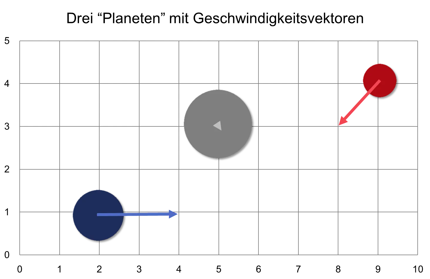
The coordinate system has a horizontal x-axis with values from 0 to 10 and a vertical y-axis with values from 0 to 5. A coordinate is given as a pair of numbers (x, y). The blue planet, for example, is located at the coordinates (2, 1).
In computer science, object-oriented programming has become the standard approach. For each planet, we need the following attributes, which together define the “state” of the object:
- a color “color”
- a mass or weight “mass”
- a position “position” in space in 2D coordinates (x, y)
- a direction-and-velocity vector “velocity” in 2D coordinates (x, y)
The direction-and-velocity vector expresses the planet’s movement. Speed is expressed by the length of the vector. Such a vector is often represented in diagrams as an arrow.
In software development, most projects use English variable names. This is partly because projects are international, partly because some employees do not speak German, and partly because the literature is in English. Only a small fraction of English-language computer science literature is translated into German. Without English, therefore, one cannot study computer science. English names are used here as well.
The following program code represents the definition of the class Circle. It is a direct implementation of the list above.
class Circle {
    String color;
    num mass;
    Vector position;
    Vector velocity;
    …
}
The program is written in the Dart programming language1. It says that there is a class called Circle with a character string (String) named “color”, a number (num) named “mass”, a vector named “position”, and a vector named “velocity” as attributes.
So-called “objects” can be created from this class. Here this is done with the function new. In the following example, the three planets are created.
var u, v, w;

u = new Circle(color: "blue", mass: 3, position: new Vector(2, 1), velocity: new Vector(2, 0));

v = new Circle(color: "gray", mass: 4, position: new Vector(5, 3), velocity: new Vector(0, 0));

w = new Circle(color: "red", mass: 2, position: new Vector(9, 4), velocity: new Vector(-1, -1));
In the program, these circles are named u, v, and w. More descriptive names could also be used, but here they should be short.
So far, the Circle class only has attributes for storing its data. But a class can also have so-called methods with which it can change the values of its own attributes. We want to calculate the new position from the old position and the velocity by adding the velocity to the current position. To do this, we have to give the Circle class a method that we call step():
class Circle {

    … as before …

    step() {
        position = position + velocity;
    }
}
A method can be recognized by the parameter list “()” and the curly braces “{}”. With step(), velocity is added to position. Before step() is called, the blue sphere has the following state:
color: blue, mass: 3, position: (2, 1), velocity: (2, 0)
After a single call, position = (2+2, 1+0)
color: blue, mass: 3, position: (4, 1), velocity: (2, 0)
And after another call:
color: blue, mass: 3, position: (6, 1), velocity: (2, 0)
It is worth noting here that the old values are lost. The Circle does not remember its history; it has no memory. That would have to be programmed separately. This is not very difficult, but it does require effort and working time. For this reason, programs are always kept as minimal as possible: they should contain only as much code as they need to fulfill their task. If this were not a simple, unimportant circle but the contents of a bank vault, the previous state should certainly be remembered. In real computer systems, important data is stored in databases, and methods are recorded in so-called logging files so that later one can check who changed what and when.
Important: Programming is cumbersome because everything must be specified exactly. Cumbersome work costs labor time and therefore money. That is why computer science tries to make programs as simple as possible and as extensive as necessary.
The step() method changes the state of the object, so it is also called a state change method. Mathematically speaking, the method expresses the difference between the two states; it is a difference function.
We have programmed a model of the three spheres and can “simulate” it by calling the step() methods for all three circles u, v, and w:
num t = 0;
while (t < 10) {
    u.step(); v.step(); w.step();
    t = t + 1;
}
To understand this program code, one has to “interpret” it line by line. The variable t stands for time and initially has the value 0. The value of this variable can be changed later. Then, in a so-called while loop, the step() methods of u, v, and w are called, and t is increased by 1. The variable t is counted upward step by step, starting from 0. At the beginning we are at time t=0, then comes t=1, then t=2, and so on. The while loop ends when t equals 10.
We have thus written a simulation. In the following figure, the changes for the first three steps are plotted:
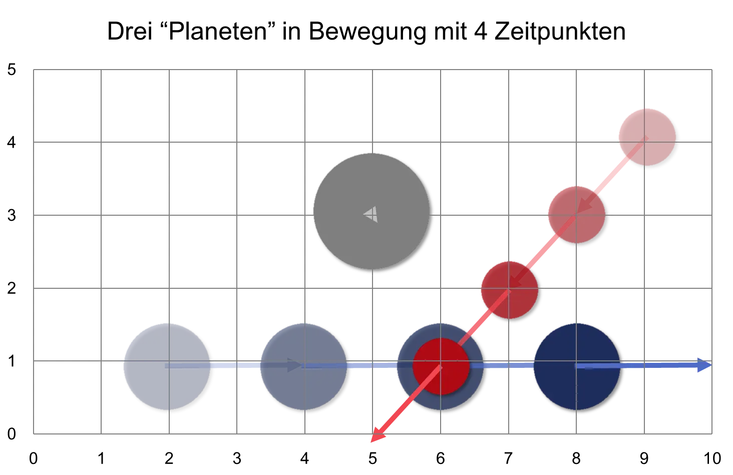
The velocity of the gray sphere is (0, 0), so it does not move. The medium-sized blue sphere moves along the x-axis because its velocity is (2, 0), and the small red sphere moves diagonally “down left” because its velocity is (-1, -1).
Now the time in variable t differs greatly from real time: natural time is continuous and does not consist of “steps.” A second can be divided into smaller parts as often as one likes. Simulated time t, however, is discrete; it consists of individual points. This is a major simplification, but it makes the model easier to program.
One could now ask whether the red and blue circles will collide. In reality, yes, but not in this model. “Collision detection” would first have to be programmed. The model does not reflect reality.
Differential Calculus
A problem with our model is that we have to calculate a great deal to find out where the spheres are at time t=1,000,000. In the simulation above, we start at t=0 and then have to call step() one million times. For large models, this can put quite a burden on the computer. Is there a faster way?
In mathematics, differential calculus has become established for this purpose. It can be used to determine a so-called closed formula for a difference function, allowing the result for any value of t to be calculated directly. For the three circles, for example, this is simple. The following three functions calculate the position of the sphere at time t without a simulation:
red(t) = (9, 4) + t * (-1,-1)

blue(t) = (2, 1) + t * (2, 0)

gray(t) = (5, 3)
Important: With a closed formula, the values for any point in time t can be calculated very easily. The simulation is not needed.
In many cases involving elaborate models, this saves an enormous amount of time. Unfortunately, however, closed formulas exist only for fairly simple difference functions or step() methods. We will come back to this later.
A “Complicated” Model
In the distant galaxy of the three circles, researchers make a new discovery: gravity. Gravity depends on a planet’s mass and distance, and it causes the other planets to be attracted. The planets influence one another. We will skip the physical theory here and adapt an existing program to our two-dimensional model [Wil13].
The step() method with gravity is somewhat more complicated. Readers who are not interested in programming can relax: this is the last code in this book. Interested readers, however, can try out and download the code on the book’s website:
step() {
    Vector force = new Vector(0, 0);
    objects
        .where( (Circle c) => c != this)
        .forEach( (Circle c) => force += bodyBodyInteraction(position, c.position, c.mass));
    velocity = velocity + new Vector(force.x / mass, force.y / mass);
    position = position + velocity;
}
In the first, simpler step() method, only the position changed. With gravity, however, the velocity changes as well. First, the forces force for all other circles in objects are added using the helper function bodyBodyInteraction(). Then a new velocity is calculated, and with it the new position.
The simulation has therefore become more complicated. The movements of one planet depend on the other planets. This simulation is the basis of the so-called n-body problem, which has many scientific applications [Wil13]:
- Simulation of planetary orbits in astronomy
- Molecular modeling of chemical molecules
- Particle systems in the simulation of water or fire
Graphs and Networks
The presentation so far has been the intuitive one from the “real” physical world. But we can also represent the model more abstractly. In our first system, we have three elements with no dependencies between them. We simply draw them side by side in the following diagram.
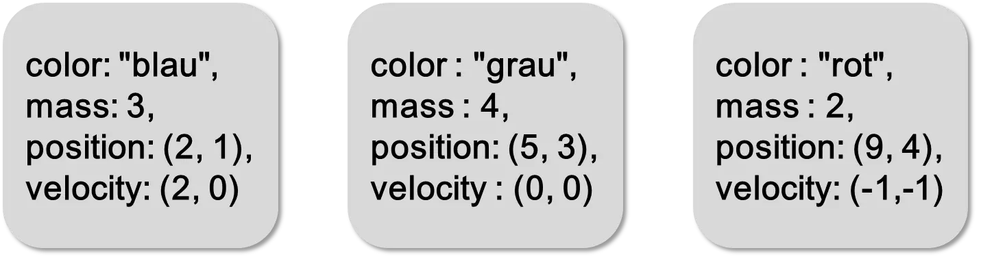
Each element has several attribute-value pairs that determine its properties or state. The individual elements are independent of one another. In the second system, gravity acted on the “planets.” In the following figure, gravity is drawn as an arrow:
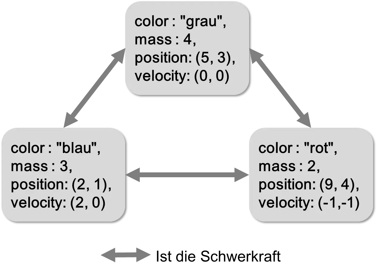
We can also draw the model a bit more abstractly and add “elements.”
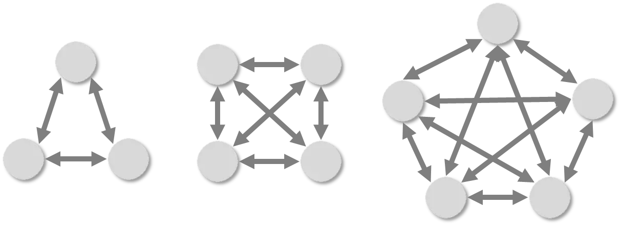
Such an abstract structure is called a graph or a network. Graphs are used in many sciences, including mathematics, computer science, the social sciences, economics, and biology. Even a city’s public-transport map or a railway route map is a graph.
A graph consists of a set of nodes (the “planets” in our simulation) and edges between these nodes, represented by the black arrows. The edges model relationships, also called relations, between the nodes. Gravity was the relationship between the individual “planets.” The last diagram, for example, contains three graphs: the graph on the left has 3 nodes and 3 edges, the middle one has 4 nodes and 6 edges, and the one on the right has 5 nodes and 10 edges.
There are different types of graphs. In the following example, the edges are “directed” and no longer bidirectional, and “loops” are allowed, so a node can be connected to itself.
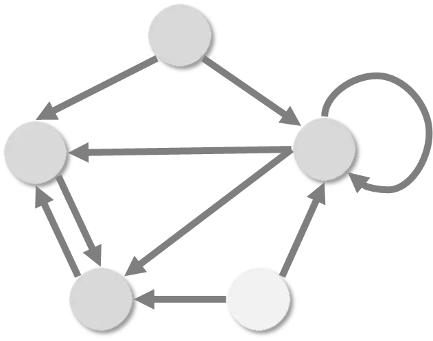
With directed graphs, it can happen that some nodes can no longer be reached by others. The light node, for example, only has “outgoing” edges; the others cannot reach it.
The advantage of the high level of abstraction in graphs is that they can be used in different fields and graph theory can be “reused.” For example, the following networks can be modeled and analyzed well with graphs:
- Technical networks: Internet, telephone network, electricity, water, gas
- Social networks: Friendships, families, acquaintances, contacts
- Economic networks: Spread of financial crises, logistics, transport
- Information networks: News, Internet, WWW
- Biological networks: Metabolic networks, transmission of epidemics, neural networks
In a social network, people are friends with one another. The following diagram shows a network with the four people Anton, Berta, Charlie, and Dennis.
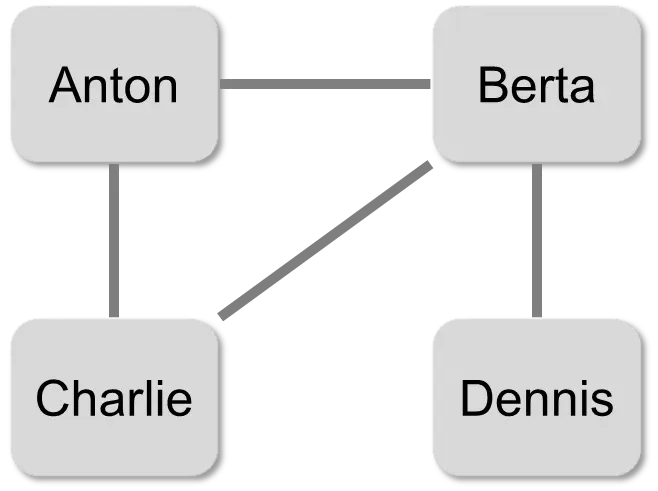
For bidirectional edges, the arrowheads are usually omitted, as they are in this graph. If two nodes are connected, then they are friends. The number of edges connected to a node is then the number of friends that person has in the network. Anton has two friends, and Berta has three.
A network can also consist of nodes of different types. In addition to people, for example, it could include cities. These different types can be visualized with different shapes or colors. In the following example, the cities are marked with darker nodes. The edges leading to these nodes are drawn as dotted lines.
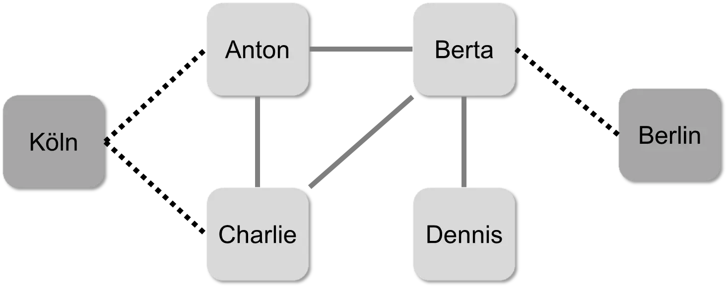
Anton and Charlie live in Cologne, Berta in Berlin, and Dennis’s place of residence is unknown.
In reality, graphs can become very complicated. Visualization programs such as Gephi2 have been developed for this purpose.
The analysis of networks is still a fairly young field, because without computers only very small networks can be analyzed. In the future, a large part of science will use network theory or graph theory.
Computer Networks
Computer networks can also be represented as graphs. The following different types of networks are the best known:
- Internet: Large international network, mostly connected via cable
- Intranet: Network connected via cable in companies or other organizations
- WLAN (“wireless local area network”): Network for smaller buildings, home network for private households
- 3G and 4G: Telecommunications networks for mobile phones
There are two main ways to connect different devices:
- Client-Server
- Peer-to-Peer (P2P)
As an example, let us assume that Anton, Berta, and Charlie want to log in to a website where they can “chat” with one another. The computer for this website is called the “server.” Anton, Berta, and Charlie use a web browser as a “client.” This architecture is therefore also called client-server architecture and is shown in the following figure.
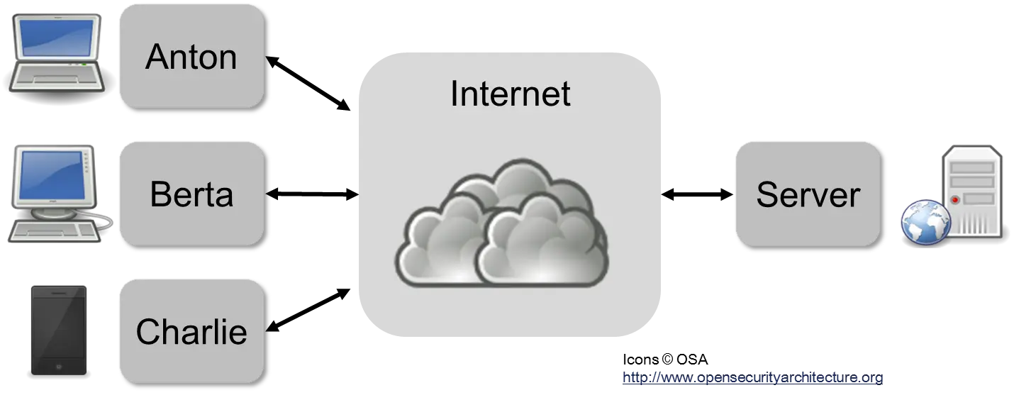
On the left side of the image are Anton with his laptop, Berta with her PC, and Charlie with his mobile phone. On the right is the WWW server. Between them is an unspecified network, often represented in diagrams as a cloud. This led to the term “cloud computing” for Internet services, such as cloud storage, where one receives storage space for data on a remote server.
Anton, Berta, and Charlie now exchange messages with one another through the server. A client-server architecture is prone to failure, because without the server communication between Anton, Berta, and Charlie does not work. In a dictatorship, such a service could easily be shut down or monitored.
An alternative is a so-called peer-to-peer network (P2P). Here, the software that was previously located on the server is distributed across all clients. Each participant is now also partly a server.
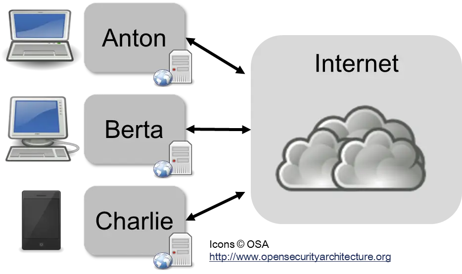
Such P2P applications, however, acquired a bad reputation because of file-sharing networks on which pirated music or films were exchanged. The P2P architecture itself is more failsafe and not easy to control. In dictatorships, it is therefore an important means of secure communication. Another example of a P2P application is the cryptocurrency Bitcoin.
A “Complex” Model
The physical system was already dynamic, but still easy to understand, because the individual planets behave deterministically according to a fixed pattern. The planets already have dependencies, but these are constant and do not change. The planets cannot decide for themselves where to fly. It becomes “complex” only when the elements make their own decisions and can adapt.
The Schelling model, named after its inventor Thomas C. Schelling, consists of m*n plots of land [Sch78]. A plot can either be vacant, or it can be occupied by a red diamond-shaped or blue square “agent”3. The field starts with a random distribution of red, blue, and empty fields. The following figure shows such a model:
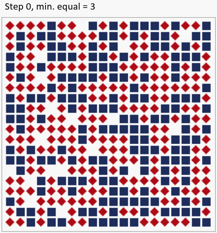
In each round, every “agent” looks at how many neighbors have the same color. If more than a certain number have a different color, the agent moves to another vacant field. An agent’s neighborhood consists of the fields around it. The following figure shows two different neighborhoods for an agent:
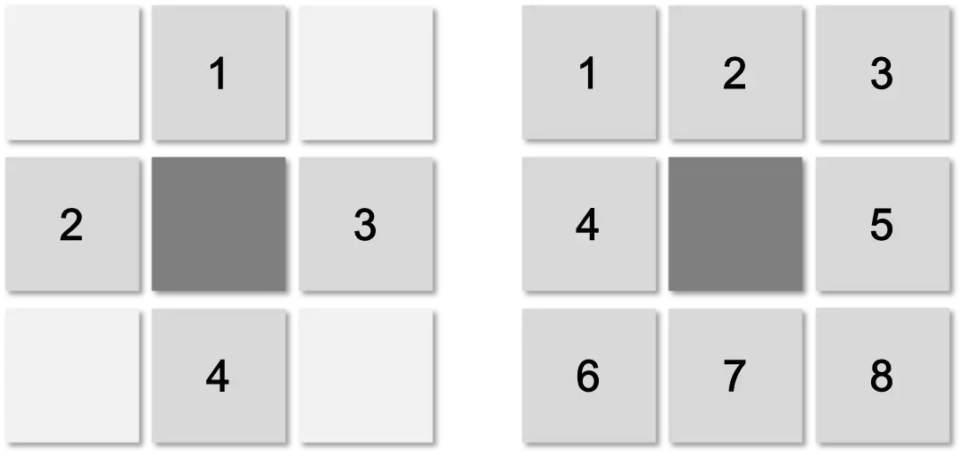
The agent is in the middle. The Moore neighborhood on the left consists only of four neighbors: above, below, left, and right. The von Neumann neighborhood also includes the diagonal neighbors4.
In our example, the agent is kept as simple as possible: in each step, he looks at his von Neumann neighborhood (with eight neighbors) and counts the different colors. If there are too few agents like him among them, he moves to some still-vacant field. We say that the agent is “adaptive”: he changes his behavior based on his environment.
Question: What does the playing field look like after a few moves, even if the agent is willing to live in a “minority” with only at least 3 similar neighbors out of 8?
Thomas C. Schelling conducted this thought experiment in the 1970s and still had to calculate it by hand. Today, it can be calculated easily with computer simulations. It can also be tried out on the book’s website. With at least three similar neighbors, the field develops as follows in the first two steps:
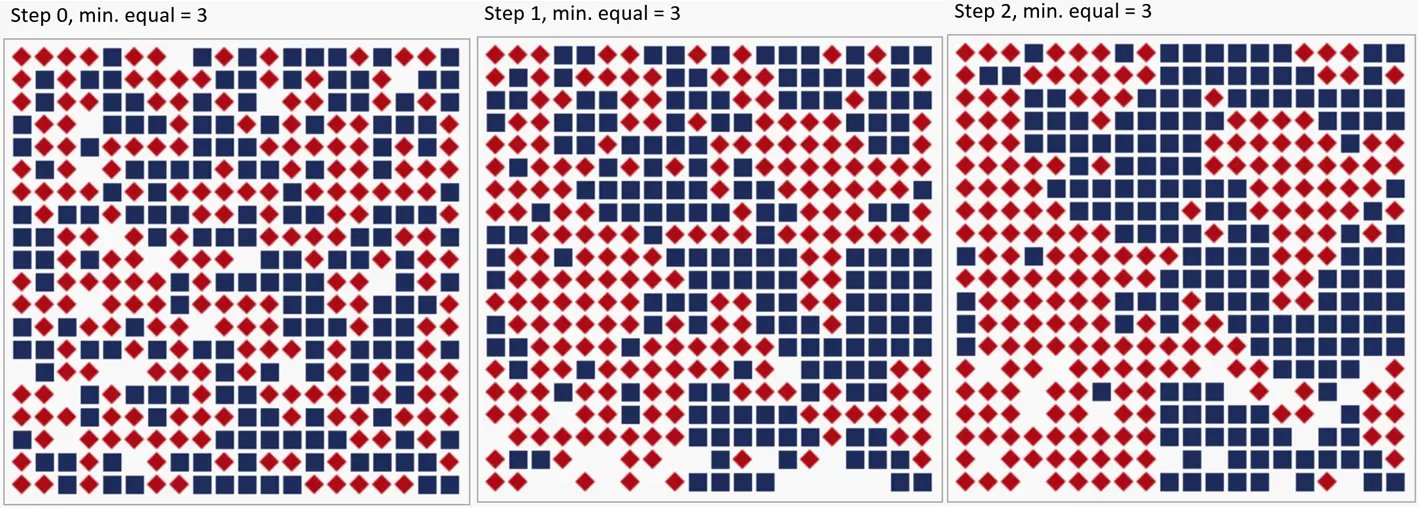
On the left is the initial situation, in the middle the first step, and on the right the second. It is already clearly visible here that the two groups are separating from one another. How can that be? After all, the agents accept living in a minority with at least three similar neighbors. Nevertheless, “residential blocks” of similar agents emerge. In sociology, this is called segregation, from the Latin for separating or setting apart.
The following figure shows the playing fields after five steps for different minimum numbers of similar neighbors: 2, 3, and 4:
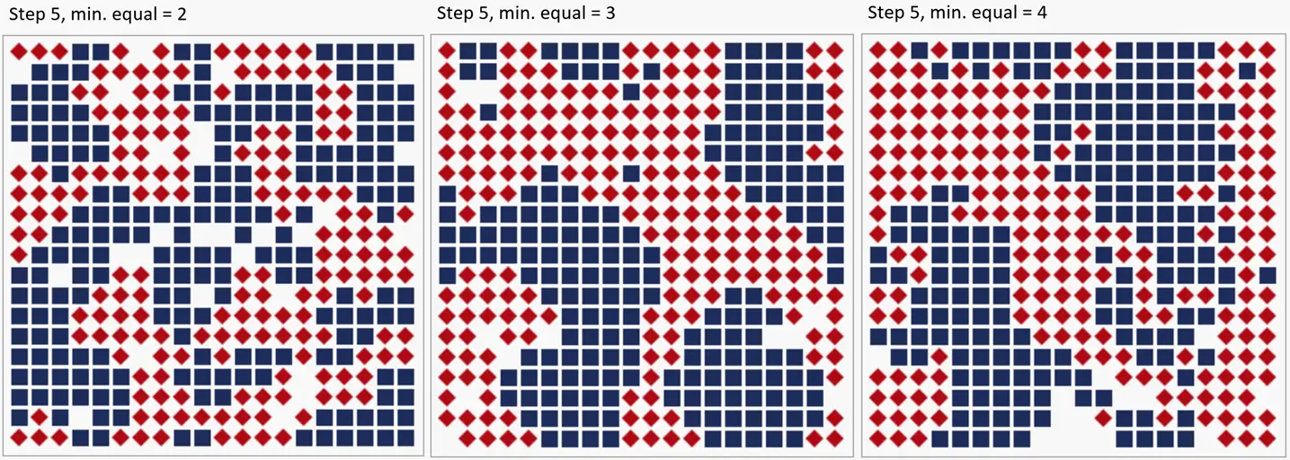
Here, too, the “blocks” are clearly recognizable. Group behavior emerges that was not “programmed in.” Critics could already accuse the society in the middle, with at least three similar neighbors, of “racism,” even though every individual agent is tolerant. In a democracy, however, a majority of 51% is always needed; that is, the agents would have to insist on at least 4 similar neighbors to reach a “draw.” At that point, however, a clear separation already appears.
The group behavior was not explicitly programmed into the individual agents; it emerged. We say that the behavior is emergent. The problem with emergent behavior is that no one foresaw it. Here the sentence “the whole is more than the sum of its parts” really makes sense5.
Important: Emergent behavior arises unexpectedly through the repetition of interactions.
The problem for science is that this emergent behavior cannot be discovered in advance. It cannot be seen by looking at the step() function. The function consists of a simple rule: “IF (number of similar neighbors <= 3) THEN move ELSE stay.” Global behavior arises from the individual local actions of the agents.
There is also a problem here for mathematicians who like to use differential calculus: so far, no solution has been found for this simple rule using differential calculus [EK10]. In the first two examples with the three “planets,” that was still possible. There, for example, one could save a million calculations because one had the closed formula. That is not possible here.
Important: A system with emergent behavior is also called a complex system. Complex systems must be simulated. Mathematics cannot describe such dynamic processes.
This example is a simple variant of the model Thomas C. Schelling had already published in 1969. Schelling was a pioneer of complex systems, and his 1978 book “Micromotives and Macrobehavior” was very influential [Sch78]. For his work in game theory, Schelling received the “Nobel Prize” in Economics in 2005 together with Robert J. Aumann6.
A model is an abstraction and a simplification of reality. Following the principle of “Ockham’s Razor,” this example is intentionally minimalist. It is the smallest model that generates segregation. This simple model can nevertheless be the starting point for further investigations, because it could be extended in various ways [EK10, Bat07, RG11, EA96, MP07]:
- More than the two different agent colors “red” and “blue”
- Larger neighborhoods: all neighbors reachable in two steps
- Different thresholds for moving: red agents move with fewer than 3 similar neighbors, blue agents with fewer than 2 similar neighbors
- The distance could be restricted during a move
- One could introduce rents or land prices
Agent-Based Modeling (ABM)
In the previous examples, we already used “agents.” Now it is time to clarify the term. An agent acts; it “does” something. The word comes from the Latin “agere” and means “to act” or “to conduct.” An agent lives in an environment and perceives information through its sensors. With its actuators, the agent can interact with the environment. An agent acts according to defined rules. In a simulation, a number of agents are “released” into an environment. In each time step, the agents are then allowed to perceive and act according to their rules. Agents form artificial societies that arise and change during a simulation. The goal of a simulation is to understand how and under what circumstances emergent behavior occurs. A “CompuTerrarium” is created [EA96].
This is also called agent-based modeling (ABM) [RG11, EA96, WR15]. It is a new way of doing science. Kenneth J. Arrow, who received the “Nobel Prize” in Economics in 1972 and discovered the famous Arrow theorem, said in 2006, “I am convinced that agent-based attempts in economics will become an important tool” [Eps06].
But ABM requires a change in thinking. Problems are formulated from the perspective of individuals, not from the perspective of the whole. The world is viewed from the “bottom,” not from the “top.” It is “bottom-up” modeling rather than “top-down” modeling. The writer Leo Tolstoy (1828 - 1910) was one of the first people to describe this “bottom-up” perspective [Eps14]. In his work “War and Peace,” he wrote the following in 1812:
“To study the laws of history, we must completely change the subject of our observation, must leave aside kings, ministers, and generals, and examine the homogeneous, infinitely small elements by which the masses are guided.”
… and …
“Only by taking an infinitely small unit for observation (the differential of history, that is, the homogeneous tendencies of men) and attaining to the art of integrating them (that is, finding the sum of these infinitely small units) can we hope to arrive at the laws of history.”
This “differential” is the step() method. But as innovative as Tolstoy was here, he was also a little mistaken, because as we now know, it is not enough “to calculate the sum of these infinitely small individual parts”; we must “simulate the product.”
ABM has already been used successfully in many different areas. Dynamic processes can be represented very well with it. ABMs have helped, for example, to clarify the following questions:
- How do social norms and customs arise? [Eps06]
- How do forest fires spread? [WR15]
- How do cities develop? [WR15, EA96, Bat07]
- How do epidemics and other diseases spread? [WR15]
- Where do traffic jams occur? [WR15]
- How can rainforests be used economically while also preserving biodiversity? [RG11]
- How do tumors grow? [WR15]
ABMs are still a fairly young development, and their use is steadily increasing. In the following sections, we will present a few ABMs.
Sugarscape
In their 1996 book “Growing Artificial Societies: Social Science from the Bottom Up,” Joshua M. Epstein and Robert Axtell created a model called “Sugarscape,” which is still often used today [EA96]. Sugarscape consists of a 2D grid of cells. In some of these cells, a random amount of sugar grows in each time step. The agents have a metabolism and require a randomly determined amount of sugar in each time step. They can harvest this sugar from the field they are currently standing on. Sugar they do not consume is kept as a reserve. At most one agent can occupy each cell. The following figure sketches a “Sugarscape”:
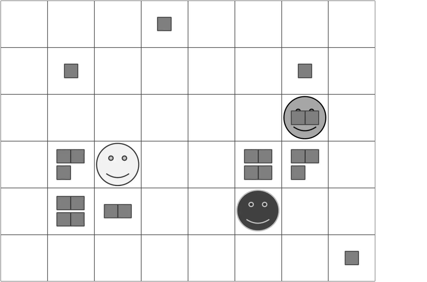
Sugar is represented by the small blocks. There are three agents: Light, Medium, and Dark. Only “Medium” has something to eat. The other two are standing on fields where there is nothing. The agents have a randomly determined visual range with which they can search their surroundings for sugar, as sketched in the next figure:
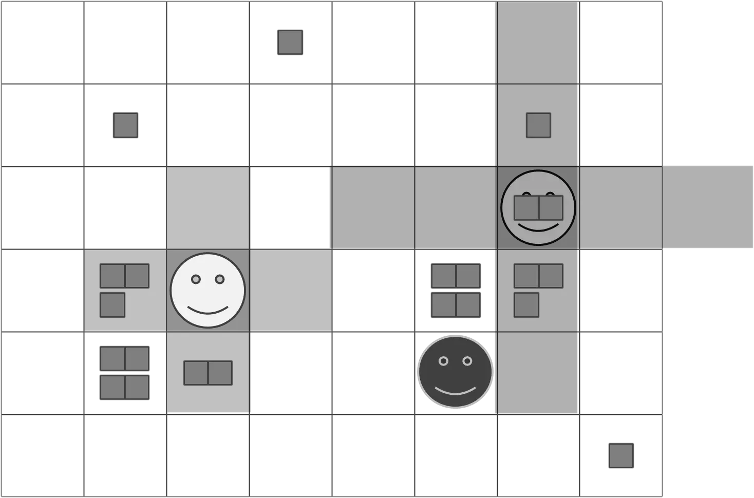
The light agent with a visual range of 1 sees only the nearest neighbors; the medium-gray agent with a visual range of 2 also sees the neighbors of the nearest neighbors. The agents cannot look diagonally; they consider their Moore neighborhood.
At the beginning of the simulation, the amount of sugar in each cell is determined. Then the agent population is defined, along with each agent’s metabolism and visual range. In the step() method, the agent carries out the following steps:
- How much sugar do I find in my surroundings within my visual range?
- Is that more sugar than on the field I am currently standing on?
- If yes, go there; otherwise stay
- Take the sugar from the current cell
- Eat enough sugar; if not enough is available, “die” and drop out
And so it continues for each time step. The following figure shows a screenshot made with the NetLogo tool.
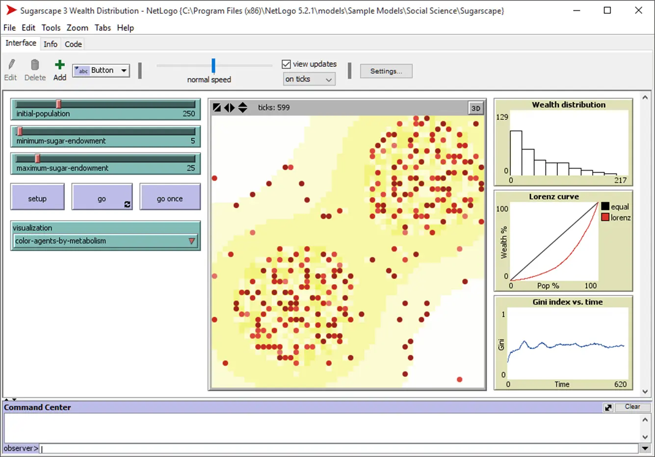
There are many possible variations here:
- The size of the field and the number of agents
- How much sugar can be on a cell?
- How fast does the sugar grow? Fast or only slowly, e.g., one piece per time step?
- Agents could have a limited lifespan. After t time steps, they then die automatically. A new agent is added randomly as a replacement.
Epstein and Axtell work through various possibilities in their book. Even in this simple “game world,” three properties known from reality can already be shown [EA96]:
First, an environment can sustain only a certain number of living beings; it has a “carrying capacity,” as in ecology. If too many agents are created, the environment can no longer feed them. This may seem trivial at first glance, but in a more complex model, one could model real agricultural systems and calculate how many people this agriculture can feed.
Second, in simulations with a large number of agents above the “carrying capacity,” it becomes clear that “selection” occurs. Agents with a wide visual range and low metabolism are more likely to survive than others.
Third, the agents can accumulate a supply of sugar; they can become wealthy. Here, the “distribution” of the agents’ wealth was analyzed and found to be a so-called Pareto distribution, named after Vilfredo Pareto (1848 - 1923). This wealth distribution is an emergent property and is shown in the following graph:
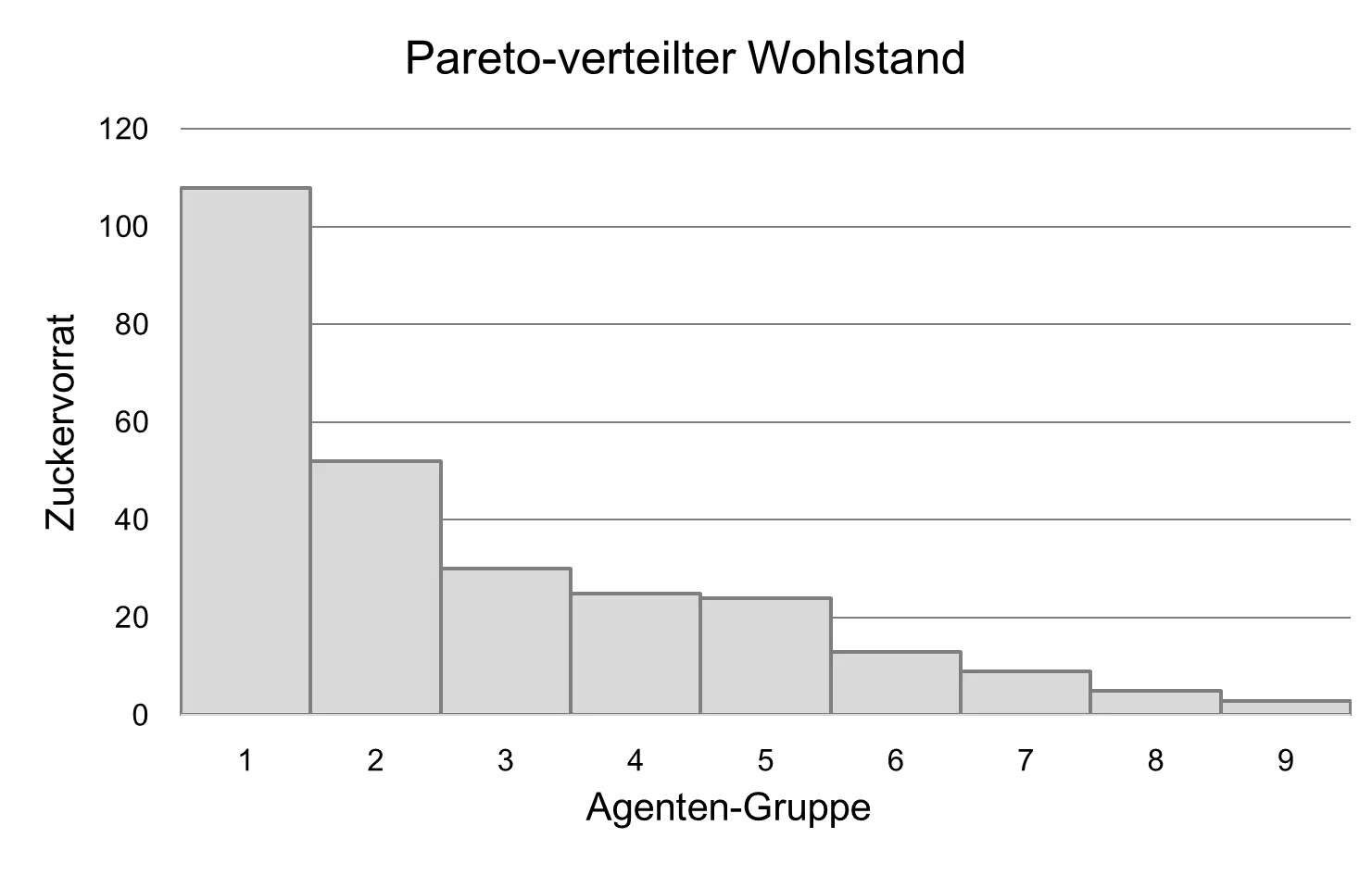
The rich agents therefore have much more sugar than the poorer ones. In other words, wealth is unequally “distributed.” Incidentally, Pareto found this distribution while examining real incomes in Italy. This type of distribution occurs in many complex systems. Another example of a Pareto distribution is the distribution of words in an English text. Some words occur much more often than others, such as “the”, “a”, “is”, “of”, and so on.
It should be noted here that the term “distribution” comes from statistics and refers to how frequently certain values occur, to how they “distribute” themselves. It does not mean that there is a “distributor” somewhere. No one carries out this distribution. If one were to call the distribution above an “unjust distribution,” that would miss the point, because no one in this model is “unjust.” No agent does anything to the others in this model. They all simply go about their own business. Complex systems have no internal or external control; they “regulate themselves.” A “spontaneous order” arises. This “order,” however, does not have to be in the observer’s interest and can also create great inequalities.
In this model, the inequalities arise because the agents have different metabolisms and visual abilities. In addition, the sugar is distributed unevenly. At the moment, the simulation follows the rule “first come, first served.” Anyone who happens to begin on a sugar-rich cell has an advantage. The emergent “bottom-up” behavior therefore produces undesirable results.
The opposite of “bottom-up” is “top-down,” and even in this simple example one can begin to consider how this economy might be adapted to one’s own ideas of “justice” through “interventions.” Is it better if everyone has the same amount of wealth? How could that be achieved? “Simply collect and distribute” sounds easier than it is, because this “redistribution” also has to be carried out by agents. One needs agents who collect sugar and distribute it to the poorer agents. But who determines how much sugar is collected and who is poor enough to receive some? Is that decided centrally for everyone? Must these “redistributors” also come with politicians and an entire democracy? The redistribution must be carried out by agents who also have to eat sugar, because they too have a metabolism. Are they allowed to eat from the collected sugar? An agent with a high metabolism could become a redistributor because that is the only way to get access to a lot of sugar.
The Sugarscape model may seem simple and trivial at first, but many political questions already arise here, and they are not at all easy to solve or implement. As a programmer, one cannot simply say at this point “the state must do that” and leave the matter there, because the state would first have to be programmed as well. And before that can be done, one has to ask, “how exactly should the state actually do that?” What means are available to it? Who pays for it? Who ensures that the “redistributors” do not constantly increase their own “stipends” (with sugar, the term “diet” takes on an entirely new flavor here).
Sugar and Spice
Over the course of their book, Epstein and Axtell examine many extensions of the basic model [EA96]:
- Migration through seasonal effects: When seasons are introduced and sugar grows more slowly in some regions, migratory movements can be observed.
- Environmental pollution: If harvesting sugar creates dirt, polluted areas emerge and the agents have great difficulty feeding themselves.
- Sexes and reproduction: If the agents are given a sex and can have children, it is possible to study which characteristics are passed on and how the population develops.
- Cultural attributes: How do certain opinions spread? How do networks arise? How do “tribes” of agents emerge?
- Aggression: What happens if aggression is allowed?
- Spice as a second good: If, in addition to sugar, there is a second commodity, “spice,” and the agents’ metabolism is changed so that agents need both to live, then barter with neighbors emerges. Economic phenomena can then be studied, such as the prices at which the two goods are traded.
All these examples make clear that complexity can be generated with very simple means. Many questions arise here that science and politics have not yet solved. But ABM can help find answers to these questions.
Why Did the Anasazi Move Away?
The “Long House Valley” in Arizona in the southwestern United States was inhabited for centuries by Anasazi Indians. But quite suddenly, around 1300 AD, the entire population left this valley, and for a long time afterward it was no longer inhabited. Some researchers suspected a period of drought as the cause.
Starting from their Sugarscape model, Epstein and Axtell developed a model of this valley [Eps06]. The valley is 96 square kilometers in size and today lies on a Navajo Indian reservation. Research had produced extensive data about the climate and environment in this valley. The valley’s climatic conditions also made it possible, for example, to investigate agricultural use in the past. Excavations provided insight into the population’s various stages of cultural development over time. Researchers had found that from 7000 to 1800 BC, hunter-gatherers sparsely populated the area. Around 1800 BC, agriculture began with the cultivation of maize and then led to the Anasazi culture, until its sudden disappearance around 1350 AD. For agriculture, geological knowledge about the condition of the soil and the occurrence of water is very important.
Data from many different projects and databases had to be brought together. It must be emphasized explicitly that this work was possible only because reusable data from earlier research existed. Without this “data collection,” the simulation would not have been possible. Researchers are also needed who understand data well enough to store it in the right scope and format. Researchers need knowledge of data and data analysis.
The simulation was calculated from 800 BC to 1350 AD. In this model, households were used as “agents” because the exact number of inhabitants and their behavior were not known, while the approximately 200 households were known from excavations.
The result of the simulation is that the entire population did not leave the valley because of a persistent drought alone. Although the valley had become drier, it would still have supported a few inhabitants. The fact that all inhabitants left the valley together must therefore also have had social reasons. The inhabitants probably did not want to separate from one another.
The model is also available in NetLogo. The following screenshot shows an excerpt from the simulation.
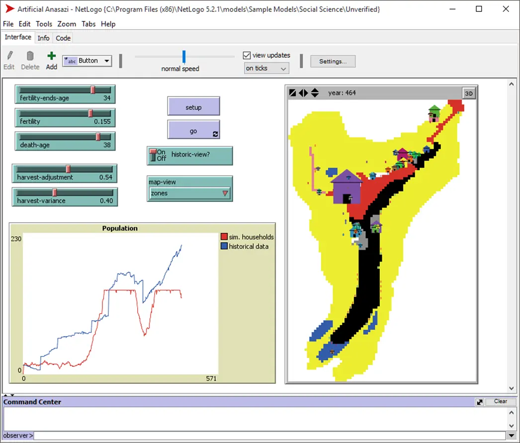
The screenshot shows that this model did not correctly predict the absolute population figures, but that was improved in a later model [Eps06, Chap. 5]. The American historian Jared Diamond wrote in the American journal Nature that this project represented a “new standard in archaeological research.”
“More Human” with Agent_Zero
In traditional agent-based modeling, agents are often quite mechanical because they only work through simple IF-THEN conditions. But social phenomena can only be studied with “more human” agents. For this reason, Joshua M. Epstein developed a “software individual,” which he presents in his book “Agent_Zero: Toward Neurocognitive Foundations for Generative Social Science” [Eps14]. Agent_Zero is intended to behave in a “more human” way, to make mistakes, and not to be a perfect “homo oeconomicus.” To this end, it has three different “components”:
- Feelings: emotional, feeling-related (“affective”)
- Thinking: cognitive, deliberative (“deliberative”)
- Social: Network with others who can influence him
These components can also disagree with one another: Agent_Zero therefore has an “inner life,” possibly even with contradictions. In this way, Agent_Zero is intended to represent the complexity of human behavior better.
Of course, this sounds better than it really is: Agent_Zero consists of three functions whose results are added together. They are relatively simple formulas, but they were designed on the basis of findings from neuroscience. In Epstein’s own view, these formulas are anything but perfect and should be understood only as a first approach. In his opinion, however, they do the job, because his goal is not to model the individual but society. When several of these simple agents “come together,” they generate the social behavior he wants to study.
For this purpose, he simulates, for example, the Arab Spring of 2011, the emergence of business cycles in the economy, or American court cases in which the hearts and minds of jurors must be won.
Complex Economics
The economist W. Brian Arthur has investigated economic problems with the help of complex systems and ABM. Since the 1980s, he has been working on “complexity economics.” For example, he has used ABM to study the following topics [Art14]:
- Manipulation of financial systems
- Behavior of stock markets
- Technological competition and economies of scale (“increasing returns”)
- How inventions work
Complex economics will be covered in more detail later in Chapter 5.
You Yourself as an Agent
You are the agent, and so are other people. The environment is the real world. What would have to be programmed into the step() function? Do you also think about vacations or retirement? If you want to buy a car, how much credit should you take out?
What would the agent have to consider? Economic behavior, certainly. But for that, one would first have to become aware of why one makes purchases the way one does. Most purchases, for example in the supermarket, are made out of habit and without much thought. Why do I buy a particular yogurt, and how do I teach the agent to do that? Traditional economics views the economy from a bird’s-eye perspective (“top-down”); it calculates aggregates and builds models with differential equations.
Agent-based modeling (ABM) requires a completely different perspective: “bottom-up.” Here, in this example, it corresponds to the first-person perspective.
Complex Systems
Classification
We have now become acquainted with various models. The examples have shown that whether a system is simple or complicated depends on several factors:
- Number of elements or nodes
- Complexity of the individual nodes, in particular the
step()function - The number and “complexity” of the relationships between the elements
Systems can be categorized colloquially as follows [Pea15]:
- Simple (“obvious”)
- Complicated (“complicated”)
- Complex (“complex”)
- Chaotic (“chaotic”)
These are not scientific definitions, but they work well in everyday use.
In a simple system, cause and effect are clearly recognizable. There are no side effects. Anyone can apply learned recipes here, as with IKEA™ or LEGO™.
In a complicated system, by contrast, analyzing cause and effect already requires effort and expert knowledge. Optimal solutions can be calculated with some effort. The knowledge needed to solve tasks in complicated systems is taught in schools and universities. Solutions arise from combining existing knowledge. A detective story is a good example here, though not the simple ones on television, but rather Agatha Christie, Ellery Queen, or John Dickson Carr.
In complex systems, the relationship between cause and effect is visible only in hindsight. Optimal solutions are very difficult to find, or they do not exist. Solving a complex system often exceeds the abilities acquired through formal education. One must invent something new or apply existing knowledge in a new way.
A chaotic system, by contrast, is a hopeless case. It is not possible to determine rationally what is cause and what is effect.
Here one must distinguish strictly between whether a system is complex and whether it is merely regarded as complex. Chess, for example, was once regarded as complex; on closer inspection, however, it is a simple mathematical optimization problem and today is considered only complicated, because creating chess programs is still complicated. Whether a system is seen as simple, complicated, or complex therefore also depends on education, knowledge, and the available technology.
Properties of Complex Systems
Complex systems show emergent behavior and often also have further special properties [Hol14, EK10, MP07, Mit09]:
- Self-organization: Complex systems have no internal or external control; they “regulate themselves.” A “spontaneous order” arises. This “order,” however, does not have to be in the observer’s interest. One example is flocks of birds.
- Adaptivity: The agents of the system adapt, and through them the whole system adapts. This adaptation can happen through learning or through evolution.
- Decentralization: There is no central control, only self-control by the individual elements.
- Each component has relatively simple rules. The overall system has complex behavior.
- Diversity: Some complex systems become even more complex over the course of their existence as the diversity of their elements increases. In a jungle, for example, new animal, insect, and plant species arise.
- Butterfly effect: Small differences in the initial configuration can have large effects and lead to completely different results. Can a butterfly in Brazil trigger a tornado in Texas? [TG15]
In some books, a distinction is made between “complex physical systems” (CPS) and “complex adaptive systems” (CAS). Others distinguish between “complex systems” and “complex adaptive systems.” For reasons of simplicity, we do not do that here.
Differential Equations
The traditional scientific tools for describing dynamic systems are differential equations. Like the step() method, they express differences with respect to time. For a passenger car, this differential is, for example, speed, given in km/h. For many simple and complicated systems in science, differential equations are often the best choice7. But they have difficulty with complex systems.
Important: Differential equations are not suitable for complex systems; these must be simulated with ABM.
Agent-Based Modeling (ABM), Part 2
ABMs therefore have many advantages over differential equations, because only rudimentary programming skills are needed and the “bottom-up” perspective is much more natural [Eps06, RG11, EA96]. ABMs are easier to understand and often offer causal explanations, while mathematical methods usually consist only of numbers and amount to “number crunching.” Another advantage of ABM is that there is a smooth transition between simulations and computer games [BP12].
The goal of agent-based modeling is to generate and investigate particular emergent behavior in systems. It is a new scientific instrument for a “generative science” and produces “generative explanations” [Eps06, WR15].
At present, however, ABMs are not yet very widespread: people have traditions and habits. If someone has already invested a great deal of time and work in one scientific method, why should he learn a second method and start again from zero? A comparison between scientific progress and a hike through a mountain range helps here [CK14]. The individual mountains represent scientific methods, and the higher one climbs, the more the mountaineer or researcher knows. Knowledge is hidden in the mountains, and the scientist searches for a way through. On the hike, he has already climbed quite far up one mountain. But then he discovers an even higher mountain in the distance, where he would gain even better insights. The problem, however, is that he would first have to descend quite a way in order to climb the higher mountain. He would therefore begin again at a lower level. Progress on the first mountain prevents or delays climbing down and continuing on the second mountain. This problem is called “Twin Peaks” in the English literature, like the legendary 1990s television series by David Lynch8.
But even if ABM is not yet very widespread today, it is important to view problems from the “complex” perspective.
For beginners, the following software tools for ABM are available, among others:
- NetLogo is a variant of the Logo programming language adapted to ABM. It is open-source, has turtle graphics, and includes many examples; see http://netlogoweb.org. Suitable introductions are the books “An Introduction to Agent-based Modeling” by Uri Wilensky and William Rand [WR15] and “Agent-Based and Individual-Based Modeling: A Practical Introduction” by Steven F. Railsback and Volker Grimm [RG11].
- Repast consists of several open-source products and offers a development environment based on Eclipse. Programming is done either in a variant of Logo called ReLogo, or in Groovy or Java; see http://repast.sourceforge.net/. Prior experience with software development in Eclipse is recommended.
- StarLogo TNG is aimed more at children learning turtle graphics and graphical elements, http://education.mit.edu/portfolio_page/starlogo-tng/.
- MASON is a library written in Java for multi-agent simulations. It is aimed more at software developers, http://cs.gmu.edu/~eclab/projects/mason/.
- AnyLogic is a commercial platform also used in industry; a version for private learning use is available for download, http://www.anylogic.com.
Interventions
Human Action in Complex Systems
In his book “The Logic of Failure,” psychologist Dietrich Dörner described the difficulties people have when dealing with complex systems [Doe03]. Dörner and his colleagues developed a computer simulation of an agricultural system in Africa. The relationships among the individual variables in this model were deliberately designed as a complex system. The “player” has dictatorial powers in the simulation, that is, he can intervene in the economy at will. He can have wells built, fertilize farmland, and so on. Dörner’s goal was to investigate how test subjects deal with such a complex system. What do they do right? What do they do wrong?
The simulation proceeds through a series of time steps. At the beginning of each time step, the player is given the opportunity to obtain information about the state of the “economy.” He can then initiate actions. The simulation then calculates the next state, and the next time step follows.
One result of the investigation is that players do not intuitively master how to handle complex systems. The following difficulties arise [Doe03]:
- After first becoming acquainted with the system, players overestimate their knowledge of it and underestimate its complexity. They are no longer self-critical enough.
- The system’s delayed feedback is also difficult. They may see negative repercussions only later, and in a completely different place. As a result, they often cannot connect cause and effect causally.
- Under time pressure, “players” begin to “overdose” their actions. The system then swings strongly in one direction; the player then steers too strongly in the opposite direction, and the problems escalate.
- Players tend to think in linear causal chains (A -> B -> C) rather than in causal networks. Therefore, they often misjudge side effects and long-term effects.
- After wrong actions, players neglect the necessary self-criticism and self-correction and continue as before, or simply delegate difficult tasks to others.
- Exponential growth is often not recognized at first. These are processes in which something grows very strongly; they will be discussed later in Section 9.1.
Dietrich Dörner compares a complex system to a game of chess in which the pieces are connected by rubber threads and influence one another. This makes it impossible to move only one piece. The player always moves other pieces as well. Sometimes it is even worse, and there are unobserved variables. Then part of the board is not visible to the player and is obscured. The player has only incomplete information [Doe03]. In complex systems, one must think holistically and always pay attention to the overall situation; one must always keep several aspects in mind, because every intervention affects more than one aspect. Dietrich Dörner summarizes it as follows: “in a world of interacting subsystems, one must think in interacting subsystems if one wants to have success.”
Important: When dealing with complex systems, “complexity” must be taken into account.
Decisions in Complex Systems
If something is wrong in a complex system and one wants to intervene “politically” and “top-down,” for example in the sugar distribution in Sugarscape in Section 2.4, then one must devise a means by which the goal can be achieved without triggering fatal side effects. In simple systems, this is quite easy:
- Think of a goal to be achieved
- What means can achieve the goal?
- What side effects does each possible means have?
- Choose the means with the lowest side effects
- Apply the means
And precisely this is not so simple in complex systems, because in step 3 the side effects can be determined only if one knows the system well. The decision in step 4 is also difficult because many criteria have to be weighed against one another. In complex systems, decisions are made harder by the following circumstances [Doe03]:
- Complexity and interconnectedness: interdependent variables
- Intransparency: not all variables are visible or measurable
- Dynamics: The system develops further and changes; it has its own momentum
- Uncertainty: Incomplete or false information about the system
There are the following sources of uncertainty:
- Unobserved variables
- Unknown dependencies of variables
- Unknown effects of actions and interventions
In the language of networks and graphs, there are therefore unknown nodes and unknown edges. In complex systems, the relationship between cause and effect is not trivial, and an action or means often has more than one effect. Decisions in complex systems are therefore also “complex decisions.” Decision theory forms the basis for optimal decisions. Based on the available information, the optimal decision is determined with the help of probability theory [Pet11]. In complex systems, however, this information is uncertain, and therefore it is very difficult to find the “right” decision. As a rule, people cannot deal with complex systems because they cannot foresee the consequences of their actions. Political “top-down” interventions should therefore be treated with caution. We will return to this later in the political chapter, in Section 11.5.
Black Swans and Antifragility
Nassim Nicholas Taleb is a philosopher, statistician, and risk analyst who has attracted attention in recent years with a series of books. For several years he worked as a financial mathematician at several Wall Street firms. He dealt with financial derivatives and hedge funds and was right at the center of “casino capitalism.”
In “The Black Swan: The Impact of the Highly Improbable” [Tal08], he shows that people are generally blind to extraordinary events. He illustrates this with the black swan. Before the discovery of Australia, people thought that all swans were white and that swans could have no other color. On the one hand, this was correct from experience, because until then only white swans had been seen. But there are, after all, other black birds, such as ravens. A black swan, however, was considered impossible. Nassim Taleb investigates this error in thinking: why do people regard something as impossible when it is actually only improbable?
For Taleb, a “black swan” is an extraordinary event that has major consequences and that people can always explain in hindsight, according to the motto “afterwards one is always wiser.” Examples of “black swans” include financial and economic crises or the attack of September 11, 2011, on the World Trade Center.
The problem is that “black swans” are usually not considered when laws and regulations are formulated. When modeling technical systems, too, it can happen that “black swans” are forgotten and not included in the model. One example is the faulty risk models before the financial crisis of 2008.
Important: In complex systems, there can be “black swans.”
In his book “Antifragility: Things That Gain from Disorder” [Tal12], Taleb divides systems into the following three classes:
- Fragile systems
- Robust systems
- Antifragile systems
A fragile system is breakable. It cannot cope with wrong inputs or actions. It depends on the absence of disturbances. Things must proceed exactly as planned, with as little deviation as possible. Typically, human-made systems are fragile.
A robust system can also cope with wrong inputs. In some robust systems, even subsystems can fail without loss of functionality. This is achieved with redundancy. In an airplane with two jet engines, one can theoretically fail. A system that can deal with errors is also called a fault-tolerant system. Here it must be kept in mind that some systems can cope with only a limited number of errors. The last jet engine, for example, must not fail as well.
An antifragile system, by contrast, gains stability from disturbances. So far, these systems are mostly found in nature. Humans cannot yet create such systems artificially. When a person trains athletically, for example by jogging, the muscles and tendons gain from the “disturbance.” The body improves through the “disturbance,” or training, and rebuilds the muscles.
When composing systems from subsystems, one must take into account that the properties of subsystems do not transfer to the overall system. The overall system can belong to a different class than its subsystems.
An overall system made of fragile redundant subsystems is, for example, robust rather than fragile. An economy as a whole is robust if the individual companies are fragile, that is, if they can become insolvent. Here, the individual fragile parts are simply replaced. A banking system, by contrast, in which the individual banks cannot become insolvent, is not robust but fragile. The banks that accumulate losses are not replaced; instead, they can continue their misconduct.
Important: If you make subsystems more robust, the overall system can become fragile.
Nassim Taleb has also dealt with complex systems and interventions [Tal12]. In “Antifragility,” he writes:
“A complex system does not require – contrary to common opinion – complicated systems, regulation methods, sophisticated political strategies. The simpler, the better … Since things are not transparent to the last detail, an intervention has unforeseen effects.”
Nassim Taleb’s insights are extremely important for modeling systems.
-
Note: The colors red and blue are of course symbolic and can stand for any difference. One could also use numbers, such as zero and one. The model originally comes from the USA, because researchers had asked themselves how Chinatowns or black neighborhoods could emerge [Sch78]. ↩
-
The neighborhoods were named after Edward F. Moore (1925 - 2003) and John von Neumann (1903 - 1957). ↩
-
Mathematically, the statement “the whole is more than the sum of its parts” is of course true. According to category theory, there are two different operations between two elements: the sum and the product. And the product is generally—colloquially speaking—the “larger” operation [Spi14]. The whole is therefore the product of its parts, not its sum. In set theory, for example, the disjoint union is an example of a sum and the Cartesian product is an example of a product. The sum of the sets {A, 1} and {B, 2} is thus {A, B, 1, 2} and the product is {(A, B), (A, 2), (1, B), (1, 2)}. The sum loses the information about where the elements come from, whether from “left” or “right”. The Cartesian product, on the other hand, retains all information. The Cartesian product is more than the disjoint sum of its parts. ↩
-
The “Nobel Prize” for Economic Sciences was put in quotation marks because the full name “Alfred Nobel Memorial Prize for Economic Sciences” is a bit unwieldy and it actually does not belong to the original “real” Nobel Prizes. ↩
-
So-called ordinary differential equations (ODE) have only one independent variable and can be solved simply (if they are linear). However, many problems have more than one independent variable and must be described with partial differential equations (PDE). These often have no simple closed solution and must be calculated for each time step. This is done today with powerful computers and is often very time- and computation-intensive and can sometimes take up entire data centers. A large part of the computing time of the Top 500 supercomputers (http://www.top500.org/) is spent solving PDEs. Solving PDEs is still a subject of research today and also a mathematical art. Many scientific articles are written on this every year. PDEs therefore have a long learning curve and require several years of mathematical study. ↩
-
Scientists who have first painstakingly worked their way into PDEs over the years naturally do not give them up so quickly. And the scientific world is also partly very conservative, partly very skeptical of new things. Therefore, ABM will only establish itself “bottom-up”, i.e., be used in private initiative and thus gain distribution. ↩