k-d-trees with Apache Spark and Scala
July 02, 2015
This article shows how to use k-d-trees with Apache Spark.
Sometimes it is useful for companies to know where exactly there customers are: are they distributed equally across the country or are there clusters. The company can use this information to improve services, acquire new customers, open new stores, etc. For this geometrical data structures are needed, that support orthogonal range queries like e. g. k-d-trees.
In this example the data from the
Stanford Network Analysis Project (SNAP) is used. The data set called
Gowalla with the file name
loc-gowalla_totalCheckins.txt.gz has the following structure:
[user]  [check-in time]       [latitude]    [longitude]    [location id]
196514  2010-07-24T13:45:06Z  53.3648119    -2.2723465833  145064
196514  2010-07-24T13:44:58Z  53.360511233  -2.276369017   1275991
196514  2010-07-24T13:44:46Z  53.3653895945 -2.2754087046  376497
196514  2010-07-24T13:44:38Z  53.3663709833 -2.2700764333  98503
For our example application we need the latitude and the longitude.
The goal was, to calculate for every user the number of other users in his neighborhood, for
example
in a 5km^2 large area. The process should be able to run in a distributed cluster. The data are saved in
HDFS. The application was testet in a virtual cluster
with 3 nodes / Apache Spark workers.
Further requirements:
- k-d-trees in Scala
- Processing of the data with Apache Spark
- Data analysis and reporting with R
 .
.
k-d-tree in Scala
A k-d-tree ist a generalization of the one dimensional search tree from Computer Science 101.
A KdTree supports a rangQuery, a range query.
sealed trait KdTree[+T] {
    def rangeQuery(range: Range): List[(Point2, T)]
}
A k-d-tree can either be a empty, a leaf or an inner node. These three definitions can be specified
in Scala inductively with case-classes.
class Nil[T] extends KdTree[T] with Serializable {
    override def rangeQuery(range: Range): List[(Point2, T)]
        = List()
}
object Nil extends Nil[Nothing]

case class Leaf[T](val p: Point2, val value: T) extends KdTree[T] with Serializable {
    override def rangeQuery(range: Range): List[(Point2, T)]
        = if (range.inRange(p)) List((p, value)) else List()

case class Node[T](val dimension: Int,
    val median: Double, val ls: KdTree[T] = Nil, val es: KdTree[T] = Nil, val hs: KdTree[T] = Nil)
    extends KdTree[T] with Serializable {

    override def rangeQuery(r: Range): List[(Point2, T)] = {
        r.compareIth(dimension, median) match {
        case (-1,  _) => hs.rangeQuery(r)
        case ( 0,  _) => es.rangeQuery(r) ++ hs.rangeQuery(r)
        case ( 1, -1) => ls.rangeQuery(r) ++ es.rangeQuery(r) ++ hs.rangeQuery(r)
        case ( 1,  0) => ls.rangeQuery(r) ++ es.rangeQuery(r)
        case ( 1,  1) => ls.rangeQuery(r)
        }
    }
}
This kind of inductive definition of algebraic datatypes is very similiar to Haskell. In my diploma thesis you'll find a thorough description and explanation of the implementation (but only in German).
Processing with Apache Spark
The data in fileSortedByUser is filtered and only the valid rows
at the time point dt are taken.
This is implemented in the function filterToLatest.
The k-d-tree kdt is created with the help of methods defined for the
resilient distributed dataset (RDD):
groupByKey() and mapValues.
The neighbors ns are created by the range query
kdt.rangeQuery(rect).
The
Haversine.neighborhood() method returns
the rectangular neighborhood.
val rdd: RDD[CheckIn] = filterToLatest(fileSortedByUser, dt)    // get all the latest checkins for dt

rdd.persist()

// build the KD tree

val ps: RDD[(Point2, CustomerId)]            = rdd.map { c => ( Point2(c.locX, c.locY), c.id ) }
val ps2: RDD[(Point2, Iterable[CustomerId])] = ps.groupByKey()
val ps3: RDD[(Point2, List[CustomerId])]     = ps2.mapValues { p => p.toList }
val ps4                                      = ps3.collect()
val kdt: KdTree[List[CustomerId]]            = KdTree.fromList(ps4)

// query for each customer in rdd

val ns : RDD[(CheckIn,Seq[(Point2, List[CustomerId])])] = rdd.map { c =>
    val loc                                  = Point2(c.locX, c.locY)
    val rect                                 = Haversine.neighborhood(loc, windowSizeInKm)
    val ps: Seq[(Point2, List[CustomerId])]  = kdt.rangeQuery(rect)
    (c, ps.filter { x => x._1 != loc })      // ignore the point at loc, this is the current row

}
// reduce to compact output format: (CustId, #Neighbours)

val ns3 = ns.map { x => (x._1.id, x._2.size )}
utils.write(dest, mkCSV("CustomerId", "number of neighbors", ns3.collect()))
The neighbors are saved in a CSV file. Remark: type information like
RDD[(Point2, CustomerId)] is not necessary in Scala, but
it helps readability and maintainability a lot.
Analysis with R
With Apache Spark one can easily create sums, aggregations and reductions. These can be plotted
in R with ggplot2.
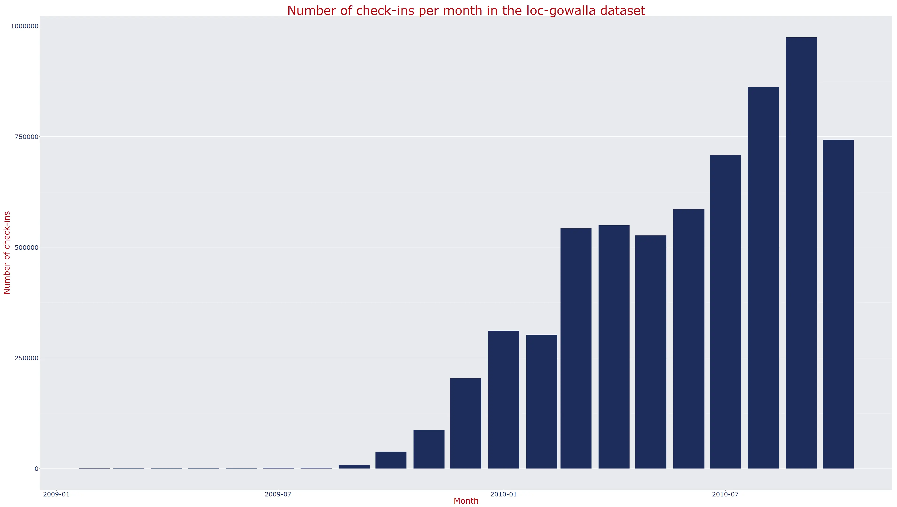
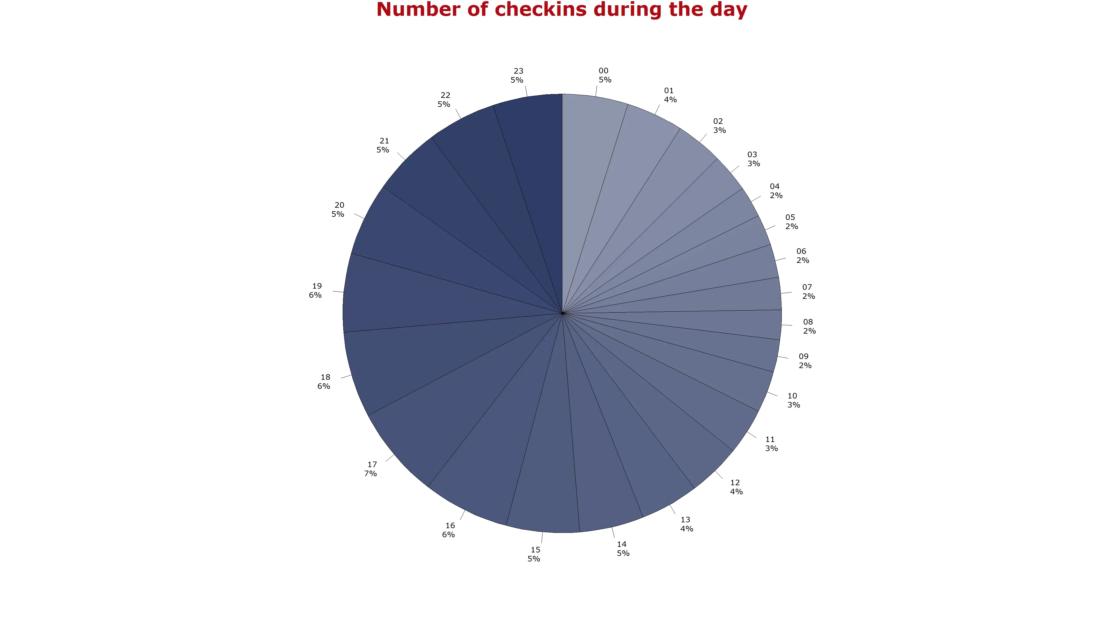
The plot on the left shows the number of check-ins per day and the simple moving average for 7 days. The graph in the middle shows the check-ins per month and the graph to thew right the check-ins per hour of the day.
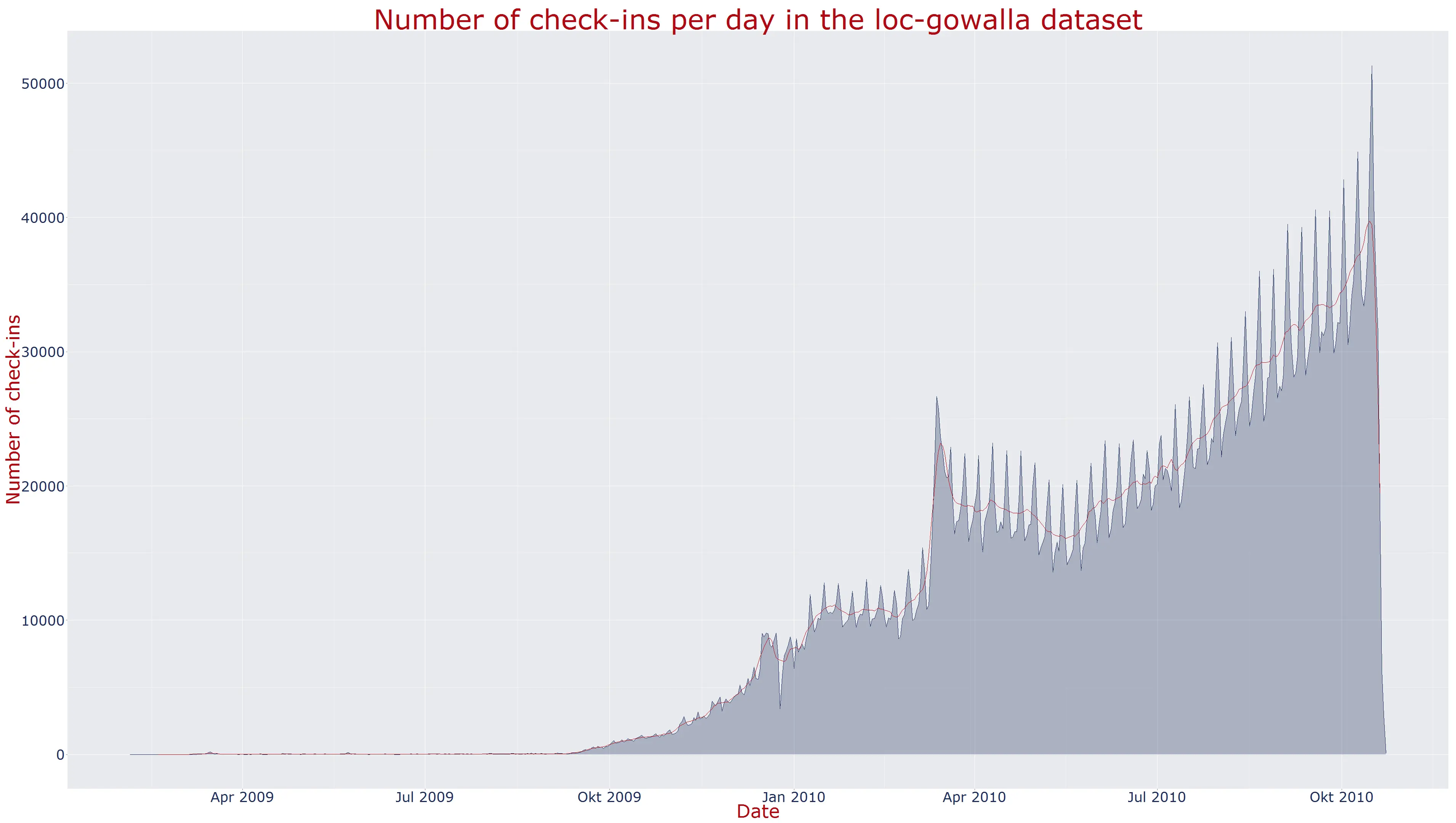
The first diagram is calculated with the folloding code (slightly simplified):
# read the csv file
a <- read.csv(file="sums_ymd.csv", header=TRUE, sep=";", colClasses=c("character", "numeric")))
a$yyyymmdd <- as.Date(a$yyyymmdd, format="%Y%m%d")
a$smoothed <- filter(a$value, rep(1/7, 7), sides=2) # smooth a 7 day time window
# create a chart with an area and two lines
ggplot(a, aes(x=yyyymmdd, y=value)) +
geom_area(fill=blue, alpha=.3) +
geom_line(color=blue) +
geom_line(aes(y=smoothed), color=red) +
theme(
panel.background=element_rect(fill=mk_color(blue, 0.1)),
legend.position=c(0.1, 0.7)) +
ggtitle("Number of check-ins per day in the loc-gowalla dataset") +
xlab("Date") + ylab("Number of check-ins") +
theme(
axis.title.x=element_text(size=12, lineheight=.9, colour=red),
axis.text.x=element_text(size=10, color=blue),
axis.title.y=element_text(size=12, lineheight=.9, colour=red),
axis.text.y=element_text(size=10, color=blue),
plot.title=element_text(size=10, color=red)
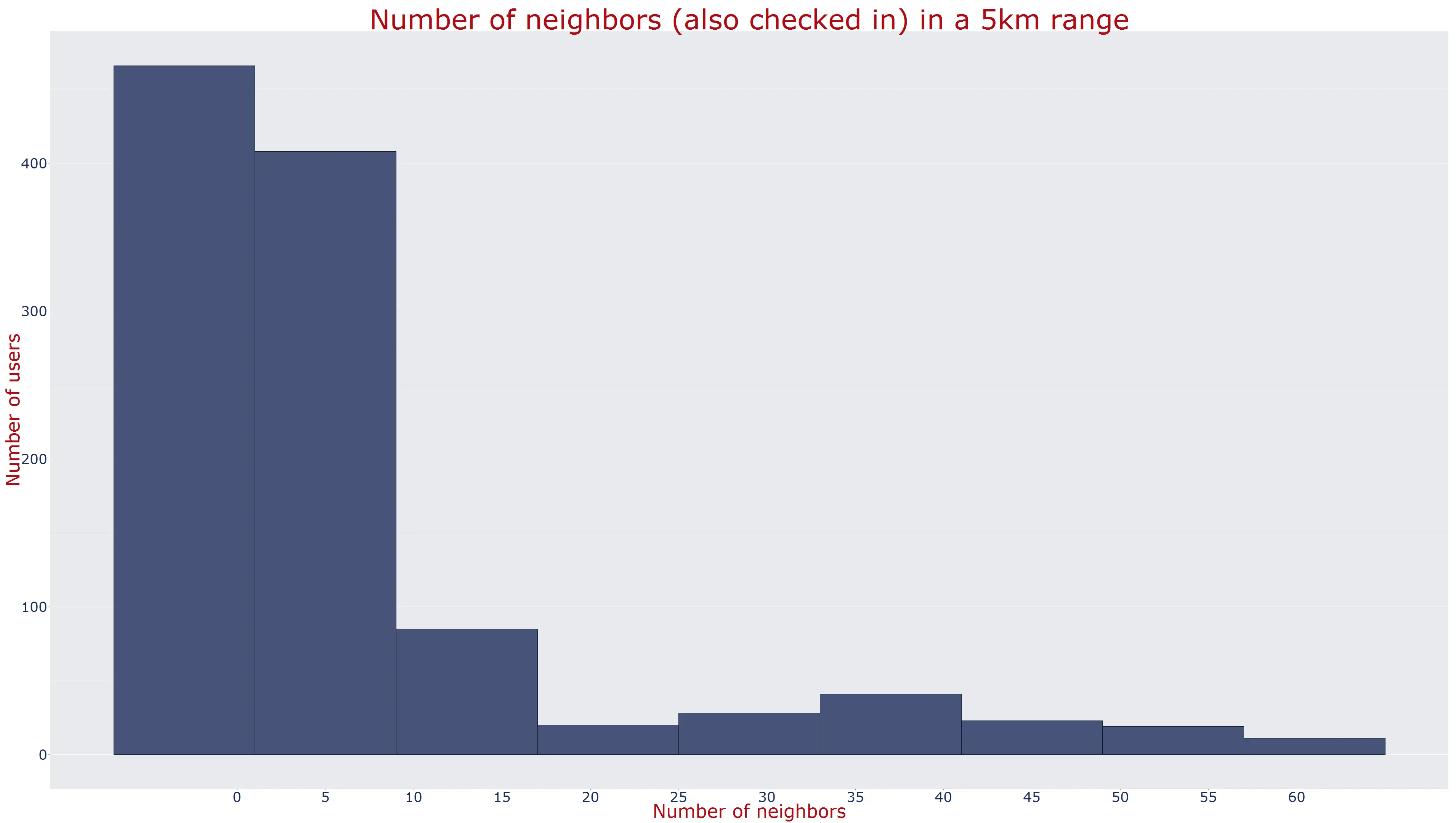
)The following histogram shows the number users that have a specific number of neighbours in a 5km^2 area.
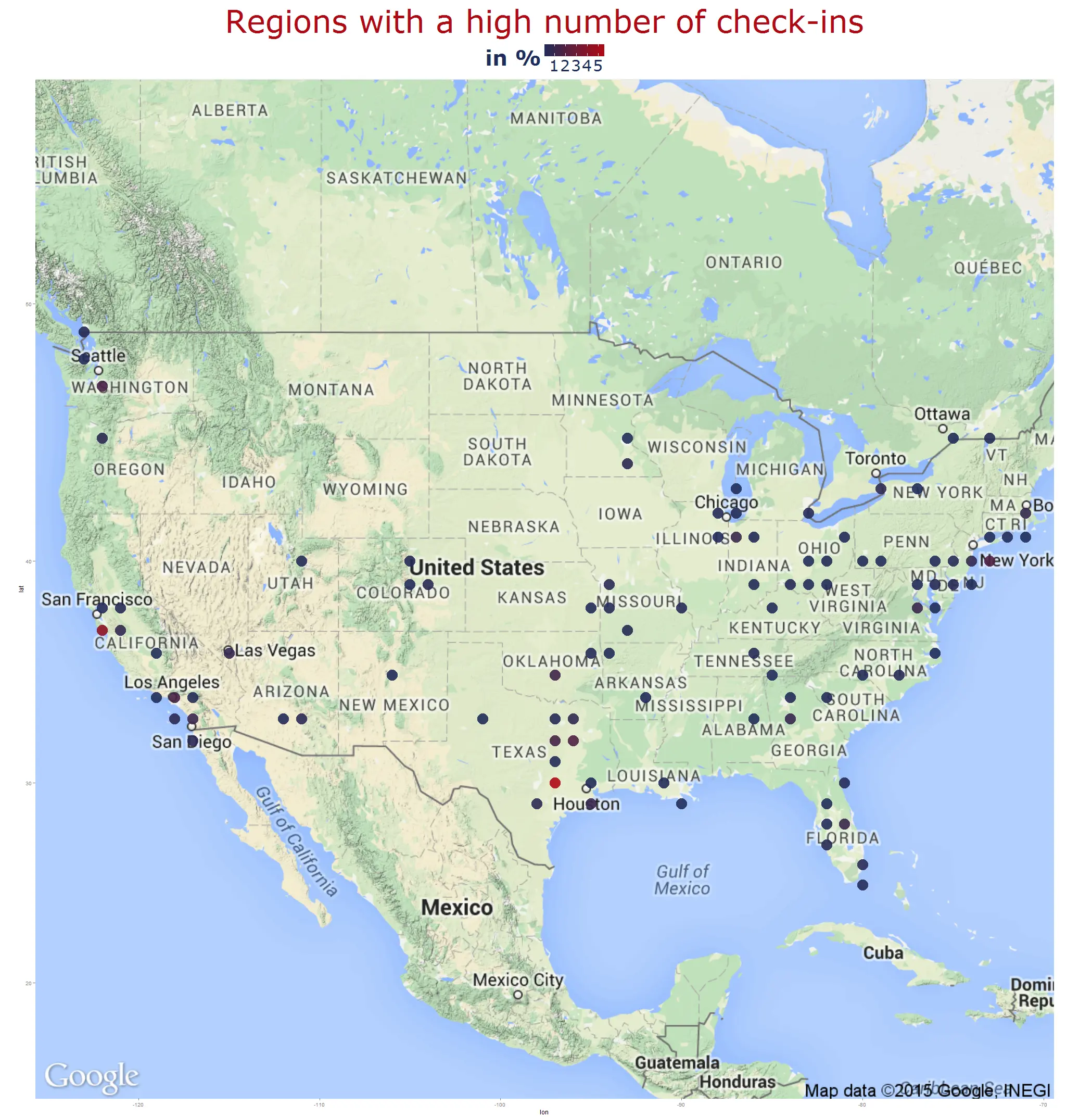
With ggmap you also can create maps with Google or
OpenStreetMap.
The following map shows the "hot spots" of people with many neighbours in red: Houston and San Francisco.
The source code is available at
GitHub
.